References:

[Images may be subject to copyright]

Motivation

It was years ago when I first came across these concepts. I decided to record it since I have been frequently deriving the entropy relations.

KLD

the concept

KLD is a method of measuring statistical distance. Sometimes referred to as “relative entropy.”
Statistical distance is the general idea of calculating the difference between statistical objects like different probability distributions for a random variable.
Kullback-Leibler divergence calculates a score that measures the divergence of one probability distribution from another.
We can think of the KL divergence as distance metric (although it isn’t symmetric) that quantifies the difference between two probability distributions.
The lower the KL divergence value, the closer the two distributions are to one another.
The KL divergence is also a key component of Gaussian Mixture Models and t-SNE.
the KL divergence is not symmetrical. a divergence is a scoring of how one distribution differs from another, where calculating the divergence for distributions P and Q would give a different score from Q and P.
Divergence scores provide shortcuts for calculating scores such as mutual information (information gain) and cross-entropy used as a loss function for classification models.
Divergence scores are also used directly as tools for understanding complex modeling problems, such as approximating a target probability distribution when optimizing generative adversarial network (GAN) models.
Two commonly used divergence scores from information theory are Kullback-Leibler Divergence and Jensen-Shannon Divergence.
Jensen-Shannon divergence extends KL divergence to calculate a symmetrical score and distance measure of one probability distribution from another.

There are many situations where we may want to compare two probability distributions.e.g., we may have a single random variable and two different probability distributions for the variable, such as a true distribution and an approximation of that distribution.
In situations like this, it can be useful to quantify the difference between the distributions.

For distributions P and Q of a continuous random variable, the Kullback-Leibler divergence is computed as an integral:

[Images may be subject to copyright]

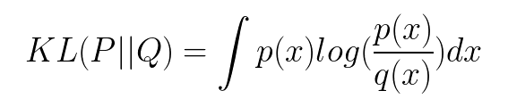
if P and Q represent the probability distribution of a discrete random variable, the Kullback-Leibler divergence is calculated as a summation:

[Images may be subject to copyright]

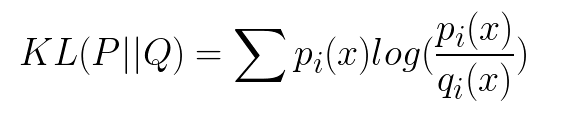
The intuition for the KL divergence score is that when the probability for an event from P is large, but the probability for the same event in Q is small, there is a large divergence. When the probability from P is small and the probability from Q is large, there is also a large divergence, but not as large as the first case.
It is like an expectation of the divergence betweent the true distribution of DGP and the approximate distribution, if you recognise the ratio (also a variable) as a measure of divergence.

The log can be base-2 to give units in “bits,” or the natural logarithm base-e with units in “nats.” When the score is 0, it suggests that both distributions are identical, otherwise the score is positive.
This sum (or integral in the case of continuous random variables) will always be positive, by the Gibbs inequality.

Importantly, the KL divergence score is not symmetrical, i.e. KL(P

Q) != KL(Q

P).

Application

If we are attempting to approximate an unknown probability distribution, then the target probability distribution from data is P and Q is our approximation of the distribution.
In this case, the KL divergence summarizes the number of additional bits (i.e. calculated with the base-2 logarithm) required to represent an event from the random variable. The better our approximation, the less additional information is required.
‘… the KL divergence is the average number of extra bits needed to encode the data, due to the fact that we used distribution q to encode the data instead of the true distribution p.’ [Page 58, Machine Learning: A Probabilistic Perspective, 2012.]

KLD Python Example 1: KL Divergence Python Example.

import libraries

import numpy as np
from scipy.stats import norm
from matplotlib import pyplot as plt
import tensorflow as tf
import seaborn as sns
sns.set()

define KLD func

def kl_divergence(p, q):
 return np.sum(np.where(p != 0, p * np.log(p / q), 0))

calculate the KLD between two close normal distributions

x = np.arange(-10, 10, 0.001)
p = norm.pdf(x, 0, 2)
q = norm.pdf(x, 2, 2)
plt.title('KL(P||Q) = %1.3f' % kl_divergence(p, q))
plt.plot(x, p)
plt.plot(x, q, c='red')

calculate the KLD between two far away normal distributions

q = norm.pdf(x, 5, 4)
plt.title('KL(P||Q) = %1.3f' % kl_divergence(p, q))
plt.plot(x, p)
plt.plot(x, q, c='red')

note that the KL divergence is not symmetrical. i.e. if we swap P and Q, the result is different:
```
plt.title('KL(Q||P) = %1.3f' % kl_divergence(q, p))
plt.plot(x, p)
plt.plot(x, q, c='red')
```

KLD Python Example 2: How to Calculate the KL Divergence for Machine Learning.

Consider a random variable with three events as different colors. We may have two different probability distributions for this variable:

1. define distributions
events = ['red', 'green', 'blue']
p = [0.10, 0.40, 0.50]
q = [0.80, 0.15, 0.05]

visulize distributions

from matplotlib import pyplot
# define distributions
events = ['red', 'green', 'blue']
p = [0.10, 0.40, 0.50]
q = [0.80, 0.15, 0.05]
print('P=%.3f Q=%.3f' % (sum(p), sum(q)))
# plot first distribution
pyplot.subplot(2,1,1)
pyplot.bar(events, p)
# plot second distribution
pyplot.subplot(2,1,2)
pyplot.bar(events, q)
# show the plot
pyplot.show()

Running the example creates a histogram for each probability distribution, allowing the probabilities for each event to be directly compared. We can see that indeed the distributions are different.

[Images may be subject to copyright]

Next, we can develop a function to calculate the KL divergence between the two distributions. We will use log base-2 to ensure the result has units in bits.
```
# calculate the kl divergence
def kl_divergence(p, q):
 return sum(p[i] * log2(p[i]/q[i]) for i in range(len(p)))
```
We can then use this function to calculate the KL divergence of P from Q, as well as the reverse, Q from P:
```
# calculate (P || Q)
kl_pq = kl_divergence(p, q)
print('KL(P || Q): %.3f bits' % kl_pq)
# calculate (Q || P)
kl_qp = kl_divergence(q, p)
print('KL(Q || P): %.3f bits' % kl_qp)
```
Running the example first calculates the divergence of P from Q as just under 2 bits, then Q from P as just over 2 bits.
KL(P || Q): 1.927 bits
KL(Q || P): 2.022 bits
This is intuitive if we consider P has large probabilities when Q is small, giving P less divergence than Q from P as Q has more small probabilities when P has large probabilities. There is more divergence in this second case.
If we change log2() to the natural logarithm log() function, the result is in nats, as follows:
KL(P || Q): 1.336 nats
KL(Q || P): 1.401 nats

The SciPy library provides the kl_div() function for calculating the KL divergence, although with a different definition as defined here. It also provides the rel_entr() function for calculating the relative entropy, which matches the definition of KL divergence here.

The rel_entr() function calculation uses the natural logarithm instead of log base-2 so the units are in nats instead of bits.

# example of calculating the kl divergence (relative entropy) with scipy
from scipy.special import rel_entr
# define distributions
p = [0.10, 0.40, 0.50]
q = [0.80, 0.15, 0.05]
# calculate (P || Q)
kl_pq = rel_entr(p, q)
print('KL(P || Q): %.3f nats' % sum(kl_pq))
# calculate (Q || P)
kl_qp = rel_entr(q, p)
print('KL(Q || P): %.3f nats' % sum(kl_qp))

Running it gives:
KL(P || Q): 1.336 nats
KL(Q || P): 1.401 nats

Jensen-Shannon Divergence

The concept

The Jensen-Shannon divergence, or JS divergence for short, is another way to quantify the difference (or similarity) between two probability distributions
It uses the KL divergence to calculate a normalized score that is symmetrical. This means that the divergence of P from Q is the same as Q from P:
JS(P || Q) == JS(Q || P)

The JS divergence can be calculated as follows:
JS(P || Q) = 1/2 * KL(P || M) + 1/2 * KL(Q || M)
Where M is calculated as:
M = 1/2 * (P + Q)

It is more useful as a measure as it provides a smoothed and normalized version of KL divergence, with scores between 0 (identical) and 1 (maximally different), when using the base-2 logarithm.
The square root of the score gives a quantity referred to as the Jensen-Shannon distance, or JS distance for short.

JSD Python example

define a function to calculate the JS divergence that uses the kl_divergence() function prepared in the previous section:
```
calculate the kl divergence

def kl_divergence(p, q): return sum(p[i] * log2(p[i]/q[i]) for i in range(len(p)))

calculate the js divergence

def js_divergence(p, q): m = 0.5 * (p + q) return 0.5 * kl_divergence(p, m) + 0.5 * kl_divergence(q, m)

2. We can then test this function using the same probability distributions used in the previous section.<br />

calculate JS(P || Q)

js_pq = js_divergence(p, q) print(‘JS(P || Q) divergence: %.3f bits’ % js_pq) print(‘JS(P || Q) distance: %.3f’ % sqrt(js_pq))

show that the divergence is symmetrical: <br />

calculate JS(Q || P)

js_qp = js_divergence(q, p) print(‘JS(Q || P) divergence: %.3f bits’ % js_qp) print(‘JS(Q || P) distance: %.3f’ % sqrt(js_qp))

Running the example shows that the JS divergence between the distributions is about 0.4 bits and that the distance is about 0.6.<br />
JS(P || Q) divergence: 0.420 bits
JS(P || Q) distance: 0.648
JS(Q || P) divergence: 0.420 bits
JS(Q || P) distance: 0.648

* The SciPy library provides an implementation of the JS distance via the jensenshannon() function. It takes arrays of probabilities across all events from each probability distribution as arguments and returns the JS distance score, not a divergence score: <br />

from scipy.spatial.distance import jensenshannon from numpy import asarray

define distributions

p = asarray([0.10, 0.40, 0.50]) q = asarray([0.80, 0.15, 0.05])

calculate JS(P || Q)

js_pq = jensenshannon(p, q, base=2) print(‘JS(P || Q) Distance: %.3f’ % js_pq)

calculate JS(Q || P)

js_qp = jensenshannon(q, p, base=2) print(‘JS(Q || P) Distance: %.3f’ % js_qp)

Running the example, we can confirm the distance score matches our manual calculation of 0.648, and that the distance calculation is symmetrical as expected: <br />
JS(P || Q) Distance: 0.648 <br />
JS(Q || P) Distance: 0.648 <br />




# Minimizing KLD
Let’s see how we could go about minimizing the KL divergence between two probability distributions using gradient descent. <br />
1. we create a probability distribution with a known mean (0) and variance (2). Then, we create another distribution with random parameters:<br />

x = np.arange(-10, 10, 0.001) p_pdf = norm.pdf(x, 0, 2).reshape(1, -1) np.random.seed(0) random_mean = np.random.randint(10, size=1) random_sigma = np.random.randint(10, size=1) random_pdf = norm.pdf(x, random_mean, random_sigma).reshape(1, -1)

2. Given that we are using gradient descent, we need to select values for the hyperparameters (i.e. step size, number of iterations).<br />

learning_rate = 0.001 epochs = 100

3. Just like numpy, in tensorflow we need to allocate memory for variables. For the variable q, we use the equation for a normal distribution given mu and sigma, only we exclude the part before the exponent since we’re normalizing the result.<br />

![Image](https://miro.medium.com/max/700/0*aPI1YDiN9lFv0RLF.jpg)
<div style="text-align: right"> [Images may be subject to copyright] </div>
<br />

p = tf.placeholder(tf.float64, shape=pdf.shape) mu = tf.Variable(np.zeros(1)) sigma = tf.Variable(np.eye(1)) normal = tf.exp(-tf.square(x - mu) / (2 * sigma)) q = normal / tf.reduce_sum(normal)

4. Just like before, we define a function to compute the KL divergence that excludes probabilities equal to zero.<br />

kl_divergence = tf.reduce_sum( tf.where(p == 0, tf.zeros(pdf.shape, tf.float64), p * tf.log(p / q)) )

5. Next, we initialize an instance of the GradientDescentOptimizer class and call the minimize method with the KL divergence function as an argument: <br />

optimizer = tf.train.GradientDescentOptimizer(learning_rate).minimize(kl_divergence)

6. Only after running tf.global_variables_initializer() will the variables hold the values we set when we declared them (i.e. tf.zeros).<br />

init = tf.global_variables_initializer()

7. All operations in tensorflow must be done within a session. In the proceeding code block, we minimize the KL divergence using gradient descent. Then, we plot the probability distribution and KL divergence at different points in time. <br />

with tf.Session() as sess: sess.run(init)

history = []
means = []
variances = []

for i in range(epochs):
    sess.run(optimizer, { p: pdf })
    
    if i % 10 == 0:
        history.append(sess.run(kl_divergence, { p: pdf }))
        means.append(sess.run(mu)[0])
        variances.append(sess.run(sigma)[0][0])

for mean, variance in zip(means, variances):
    q_pdf = norm.pdf(x, mean, np.sqrt(variance))
    plt.plot(x, q_pdf.reshape(-1, 1), c='red') plt.title('KL(P||Q) = %1.3f' % history[-1])
plt.plot(x, p_pdf.reshape(-1, 1), linewidth=3)
plt.show()

plt.plot(history)
plt.show()

sess.close() ```

Kullback-Leibler (KL) Divergence and Jensen-Shannon Divergence

A revisit to KLD and JSD

Kullback-Leibler (KL) Divergence and Jensen-Shannon Divergence

A revisit to KLD and JSD

Motivation

KLD

the concept

Application

KLD Python Example 1: KL Divergence Python Example.

KLD Python Example 2: How to Calculate the KL Divergence for Machine Learning.

Jensen-Shannon Divergence

The concept

JSD Python example

calculate the kl divergence

calculate the js divergence

calculate JS(P || Q)

calculate JS(Q || P)

define distributions

calculate JS(P || Q)

calculate JS(Q || P)